Maps and weather data

To simulate a region, Persefone.jl requires different input files:

1. A map file in the GeoPackage format, containing land cover polygons with an associated soil type.
2. A CSV file containing daily weather data for the simulated time period.
3. Regionally calibrated crop parameters for the AquaCrop model (if available).

How to calibrate AquaCrop is explained in detail here. If there are no regional parameters available, Persefone.jl will instead instantiate AquaCrop with national-level parameters.

This page will describe how the map and weather data are structured, obtained, and processed. All region data files are stored using the following convention:

data/regions/<regionname>/
-> <regionname>.geojson
-> landscape.gpkg
-> weather.csv

Where <regionname> is currently one of bodensee, eichsfeld, hohenlohe, jena, oberrhein, or thueringer_becken.

Generating input data

The process of downloading and processing map and weather data for the existing regions is fully automated. Simply execute make regions, or run the script data/regions/auxiliary/createinputs.sh.

If you only need to generate an individual region, or only weather or map data, you can use the scripts in the data/regions/auxiliary folder: extract_weather_data.R and vector_maps.jl. Note that generating map files can take a long time!

To add a new region within Germany, you must create a GeoJSON file containing a single rectangle delineating the landscape extent, and add the relevant details for the region to the two scripts listed above. Adding a region outside Germany is possible too, but in this case the input files must be created manually.

Land cover maps

Persefone.jl works with vector maps in which each geographical element is assigned to one of 32 land cover types:

@enum LandCover begin
    NoData                 # 0
    ResidentialBuildings   # 1
    IndustrialBuildings    # 2
    PublicBuildings        # 3
    OtherBuildings         # 4
    IndustrialArea         # 5
    ParkOrGarden           # 6
    Arable                 # 7
    Grassland              # 8
    Orchard                # 9
    Horticulture           # 10
    FruitPlantation        # 11
    ConiferousForest       # 12
    BroadleavedForest      # 13
    MixedForest            # 14
    TreePlantation         # 15
    Hedge                  # 16
    Scrub                  # 17
    Trees                  # 18
    Reeds                  # 19
    BareGround             # 20
    Heath                  # 21
    Peatland               # 22
    Swamp                  # 23
    RockOrCliff            # 24
    SlopeOrDike            # 25
    Stream                 # 26
    Lake                   # 27
    Ocean                  # 28
    Railway                # 29
    Path                   # 30
    Road                   # 31
end

While these maps could be created by hand using normal GIS software, it is easier to generate them from existing official cartographical maps. For Germany, these are available in the ATKIS data provided by each state (e.g. Baden-Württemberg). These maps cover all of Germany seamlessly with an accuracy of +/- 3m and are updated regularly. However, they use a complicated classification scheme that goes beyond the requirements of Persefone.jl. Therefore, the vector_maps.jl script takes these data, crops them to the desired extent, and converts the ATKIS classification to the land cover types listed above. The resulting GeoPackage file can then be copied into the respective region folder and used as input to the model.

Soil data

Soil data for Germany is provided by the Bundesanstalt für Geowissenschaften und Rohstoffe in form of the Bodenatlas. This provides a (coarse, but for our purposes sufficient) map of the distribution of the basic soil types such as clay, silt, sand, and loam.

The required map can be downloaded here. Its integer values map onto the Persefone.jl SoilType enum as follows:

1: Abbauflächen -> nosoil
2: Gewässer -> nosoil
3: Lehmsande (ls) -> loamy_sand
4: Lehmschluffe (lu) -> silt_loam
5: Moore -> nosoil
6: Normallehme (ll) -> loam
7: Reinsande (ss) -> sand
8: Sandlehme (sl) -> sandy_loam
9: Schluffsande (us) -> sandy_loam
10: Schlufftone (ut) -> silty_clay
11: Siedlung -> nosoil
12: Tonlehme (tl) -> clay_loam
13: Tonschluffe (tu) -> silty_clay_loam
14: Watt -> nosoil

The vector_maps.jl script will take this map and extract all relevant data, so that the resulting GPKG file contains soil as well as land cover data.

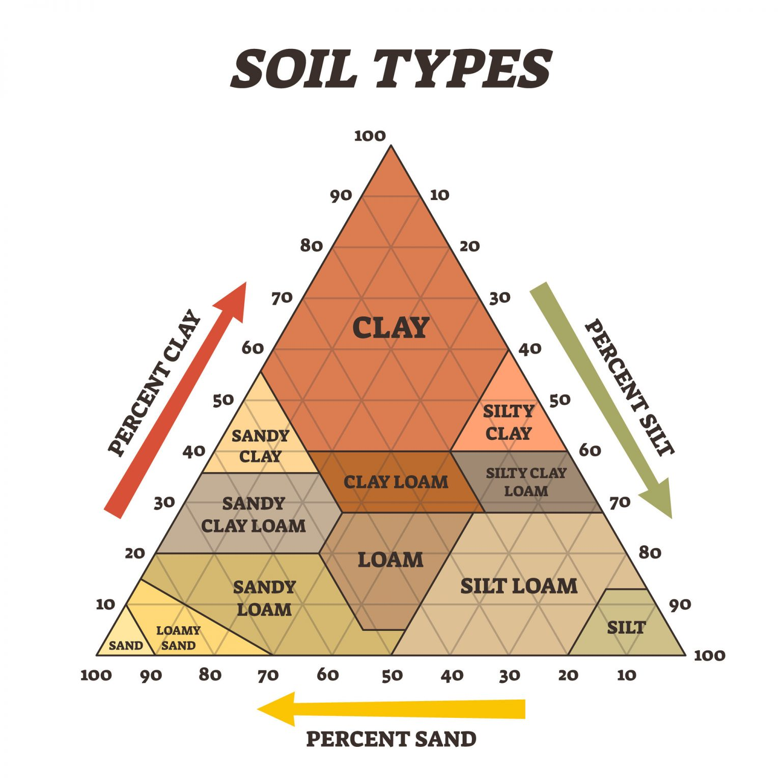
Names of soil types are based on the relative composition of clay, silt, and sand. Note that the typology used in the Bodenatlas does not map perfectly on to this international classification. Image source: Australian Environmental Education

Weather data

Currently, Persefone uses historical weather data from the closest weather station as its weather input. (In future, this may be changed to a more detailed raster input, which could then also provide future weather predictions under climate change.) Weather data can be downloaded from the German weather service (DWD).

The description of these data sets and the list of weather stations can be found in the Persefone repository, in the docs folder (or downloaded from the link above). Using the list of weather stations, select the one closest to the area of study. Note that not all stations were continuously in operation; make sure that the selected station covers the years of interest. The currently included regions have the following station codes:

• Region Jena: station number 02444 ("Jena (Sternwarte)")
• Region Eichsfeld: station number 02925 ("Leinefelde")
• Region Thüringer Becken: station number 00896 ("Dachwig")
• Region Hohenlohe: station number 03761 ("Oehringen")
• Region Bodensee: station number 06263 ("Singen")
• Region Oberrhein: station number 05275 ("Waghäusel-Kirrlach")

The extract_weather_data.R script can be used to download and process the data into the format needed by Persefone. This uses the rdwd package. To use it, simply specify the desired region, adding its ID to the stationid list if necessary. The produced CSV file can be copied into the respective region folder.